How To Draw A Mohr's Circle

Geometric civil technology adding technique

Effigy 1. Mohr'south circles for a three-dimensional land of stress

Mohr's circle is a two-dimensional graphical representation of the transformation law for the Cauchy stress tensor.

Mohr's circle is often used in calculations relating to mechanical engineering for materials' force, geotechnical engineering for force of soils, and structural engineering for strength of built structures. It is also used for calculating stresses in many planes by reducing them to vertical and horizontal components. These are called principal planes in which principal stresses are calculated; Mohr's circle can also be used to detect the principal planes and the principal stresses in a graphical representation, and is one of the easiest ways to do so.^[1]

After performing a stress analysis on a material torso assumed every bit a continuum, the components of the Cauchy stress tensor at a item cloth point are known with respect to a coordinate system. The Mohr circle is then used to determine graphically the stress components acting on a rotated coordinate system, i.eastward., acting on a differently oriented plane passing through that point.

The abscissa and ordinate ( ${\displaystyle \sigma _{\mathrm {n} }}$ , ${\displaystyle \tau _{\mathrm {due north} }}$ ) of each point on the circle are the magnitudes of the normal stress and shear stress components, respectively, interim on the rotated coordinate organization. In other words, the circle is the locus of points that represent the country of stress on private planes at all their orientations, where the axes represent the principal axes of the stress chemical element.

19th-century German engineer Karl Culmann was the first to conceive a graphical representation for stresses while because longitudinal and vertical stresses in horizontal beams during bending. His work inspired boyfriend High german engineer Christian Otto Mohr (the circle'south namesake), who extended it to both 2- and iii-dimensional stresses and adult a failure benchmark based on the stress circle.^[two]

Alternative graphical methods for the representation of the stress country at a point include the Lamé's stress ellipsoid and Cauchy'south stress quadric.

The Mohr circle can be practical to any symmetric 2x2 tensor matrix, including the strain and moment of inertia tensors.

Motivation [edit]

Figure two. Stress in a loaded deformable material trunk assumed as a continuum.

Internal forces are produced between the particles of a deformable object, causeless as a continuum, as a reaction to applied external forces, i.east., either surface forces or body forces. This reaction follows from Euler'southward laws of motility for a continuum, which are equivalent to Newton's laws of motility for a particle. A measure of the intensity of these internal forces is called stress. Because the object is assumed as a continuum, these internal forces are distributed continuously within the volume of the object.

In engineering, e.g., structural, mechanical, or geotechnical, the stress distribution inside an object, for instance stresses in a stone mass around a tunnel, airplane wings, or building columns, is determined through a stress analysis. Calculating the stress distribution implies the determination of stresses at every point (cloth particle) in the object. According to Cauchy, the stress at any point in an object (Figure two), assumed every bit a continuum, is completely defined by the 9 stress components ${\displaystyle \sigma _{ij}}$ of a 2d gild tensor of type (ii,0) known every bit the Cauchy stress tensor, ${\displaystyle {\boldsymbol {\sigma }}}$ :

${\displaystyle {\boldsymbol {\sigma }}=\left[{\begin{matrix}\sigma _{xi}&\sigma _{12}&\sigma _{13}\\\sigma _{21}&\sigma _{22}&\sigma _{23}\\\sigma _{31}&\sigma _{32}&\sigma _{33}\\\end{matrix}}\right]\equiv \left[{\brainstorm{matrix}\sigma _{xx}&\sigma _{xy}&\sigma _{xz}\\\sigma _{yx}&\sigma _{yy}&\sigma _{yz}\\\sigma _{zx}&\sigma _{zy}&\sigma _{zz}\\\terminate{matrix}}\correct]\equiv \left[{\begin{matrix}\sigma _{x}&\tau _{xy}&\tau _{xz}\\\tau _{yx}&\sigma _{y}&\tau _{yz}\\\tau _{zx}&\tau _{zy}&\sigma _{z}\\\terminate{matrix}}\correct]}$

Figure 3. Stress transformation at a bespeak in a continuum under aeroplane stress weather.

After the stress distribution within the object has been determined with respect to a coordinate arrangement ${\displaystyle (ten,y)}$ , information technology may be necessary to summate the components of the stress tensor at a particular cloth betoken ${\displaystyle P}$ with respect to a rotated coordinate organization ${\displaystyle (x',y')}$ , i.due east., the stresses acting on a plane with a dissimilar orientation passing through that point of interest —forming an angle with the coordinate system ${\displaystyle (10,y)}$ (Effigy iii). For example, it is of interest to find the maximum normal stress and maximum shear stress, likewise as the orientation of the planes where they act upon. To achieve this, information technology is necessary to perform a tensor transformation under a rotation of the coordinate organization. From the definition of tensor, the Cauchy stress tensor obeys the tensor transformation law. A graphical representation of this transformation police for the Cauchy stress tensor is the Mohr circumvolve for stress.

Mohr's circumvolve for ii-dimensional state of stress [edit]

Figure 4. Stress components at a plane passing through a point in a continuum under plane stress conditions.

In two dimensions, the stress tensor at a given material point ${\displaystyle P}$ with respect to any two perpendicular directions is completely defined by only three stress components. For the particular coordinate arrangement ${\displaystyle (x,y)}$ these stress components are: the normal stresses ${\displaystyle \sigma _{x}}$ and ${\displaystyle \sigma _{y}}$ , and the shear stress ${\displaystyle \tau _{xy}}$ . From the balance of angular momentum, the symmetry of the Cauchy stress tensor tin can be demonstrated. This symmetry implies that ${\displaystyle \tau _{xy}=\tau _{yx}}$ . Thus, the Cauchy stress tensor can be written as:

${\displaystyle {\boldsymbol {\sigma }}=\left[{\begin{matrix}\sigma _{x}&\tau _{xy}&0\\\tau _{xy}&\sigma _{y}&0\\0&0&0\\\end{matrix}}\right]\equiv \left[{\begin{matrix}\sigma _{x}&\tau _{xy}\\\tau _{xy}&\sigma _{y}\\\finish{matrix}}\right]}$

The objective is to use the Mohr circle to observe the stress components ${\displaystyle \sigma _{\mathrm {north} }}$ and ${\displaystyle \tau _{\mathrm {n} }}$ on a rotated coordinate system ${\displaystyle (ten',y')}$ , i.e., on a differently oriented plane passing through ${\displaystyle P}$ and perpendicular to the ${\displaystyle x}$ - ${\displaystyle y}$ aeroplane (Figure 4). The rotated coordinate system ${\displaystyle (x',y')}$ makes an angle ${\displaystyle \theta }$ with the original coordinate system ${\displaystyle (x,y)}$ .

Equation of the Mohr circle [edit]

To derive the equation of the Mohr circle for the ii-dimensional cases of airplane stress and plane strain, first consider a two-dimensional minute fabric chemical element around a material point ${\displaystyle P}$ (Figure four), with a unit of measurement area in the direction parallel to the ${\displaystyle y}$ - ${\displaystyle z}$ aeroplane, i.due east., perpendicular to the folio or screen.

From equilibrium of forces on the infinitesimal element, the magnitudes of the normal stress ${\displaystyle \sigma _{\mathrm {due north} }}$ and the shear stress ${\displaystyle \tau _{\mathrm {northward} }}$ are given by:

${\displaystyle \sigma _{\mathrm {due north} }={\frac {1}{2}}(\sigma _{x}+\sigma _{y})+{\frac {1}{two}}(\sigma _{x}-\sigma _{y})\cos two\theta +\tau _{xy}\sin ii\theta }$

${\displaystyle \tau _{\mathrm {due north} }=-{\frac {one}{2}}(\sigma _{x}-\sigma _{y})\sin 2\theta +\tau _{xy}\cos 2\theta }$

Derivation of Mohr's circumvolve parametric equations - Equilibrium of forces

From equilibrium of forces in the direction of ${\displaystyle \sigma _{\mathrm {n} }}$ ( ${\displaystyle x'}$ -axis) (Effigy iv), and knowing that the expanse of the plane where ${\displaystyle \sigma _{\mathrm {n} }}$ acts is ${\displaystyle dA}$ , we have: ${\displaystyle \ {\begin{aligned}\sum F_{x'}&=\sigma _{\mathrm {n} }dA-\sigma _{10}dA\cos ^{2}\theta -\sigma _{y}dA\sin ^{2}\theta -\tau _{xy}dA\cos \theta \sin \theta -\tau _{xy}dA\sin \theta \cos \theta =0\\\sigma _{\mathrm {n} }&=\sigma _{x}\cos ^{ii}\theta +\sigma _{y}\sin ^{2}\theta +ii\tau _{xy}\sin \theta \cos \theta \\\end{aligned}}}$ Yet, knowing that ${\displaystyle \cos ^{2}\theta ={\frac {1+\cos 2\theta }{2}},\qquad \sin ^{2}\theta ={\frac {1-\cos 2\theta }{two}}\qquad {\text{and}}\qquad \sin 2\theta =2\sin \theta \cos \theta }$ we obtain ${\displaystyle \sigma _{\mathrm {north} }={\frac {1}{ii}}(\sigma _{ten}+\sigma _{y})+{\frac {ane}{2}}(\sigma _{x}-\sigma _{y})\cos two\theta +\tau _{xy}\sin 2\theta }$ At present, from equilibrium of forces in the direction of ${\displaystyle \tau _{\mathrm {n} }}$ ( ${\displaystyle y'}$ -axis) (Effigy 4), and knowing that the surface area of the plane where ${\displaystyle \tau _{\mathrm {n} }}$ acts is ${\displaystyle dA}$ , we have: ${\displaystyle \ {\begin{aligned}\sum F_{y'}&=\tau _{\mathrm {n} }dA+\sigma _{x}dA\cos \theta \sin \theta -\sigma _{y}dA\sin \theta \cos \theta -\tau _{xy}dA\cos ^{2}\theta +\tau _{xy}dA\sin ^{2}\theta =0\\\tau _{\mathrm {n} }&=-(\sigma _{x}-\sigma _{y})\sin \theta \cos \theta +\tau _{xy}\left(\cos ^{2}\theta -\sin ^{ii}\theta \right)\\\end{aligned}}}$ However, knowing that ${\displaystyle \cos ^{2}\theta -\sin ^{ii}\theta =\cos two\theta \qquad {\text{and}}\qquad \sin 2\theta =two\sin \theta \cos \theta }$ we obtain ${\displaystyle \tau _{\mathrm {n} }=-{\frac {ane}{2}}(\sigma _{ten}-\sigma _{y})\sin 2\theta +\tau _{xy}\cos two\theta }$

Both equations can as well exist obtained by applying the tensor transformation constabulary on the known Cauchy stress tensor, which is equivalent to performing the static equilibrium of forces in the direction of ${\displaystyle \sigma _{\mathrm {due north} }}$ and ${\displaystyle \tau _{\mathrm {north} }}$ .

Derivation of Mohr'south circle parametric equations - Tensor transformation

The stress tensor transformation law tin be stated every bit ${\displaystyle {\begin{aligned}{\boldsymbol {\sigma }}'&=\mathbf {A} {\boldsymbol {\sigma }}\mathbf {A} ^{T}\\\left[{\begin{matrix}\sigma _{ten'}&\tau _{x'y'}\\\tau _{y'x'}&\sigma _{y'}\\\end{matrix}}\right]&=\left[{\begin{matrix}a_{x}&a_{xy}\\a_{yx}&a_{y}\\\end{matrix}}\right]\left[{\begin{matrix}\sigma _{x}&\tau _{xy}\\\tau _{yx}&\sigma _{y}\\\end{matrix}}\right]\left[{\begin{matrix}a_{10}&a_{yx}\\a_{xy}&a_{y}\\\end{matrix}}\right]\\&=\left[{\begin{matrix}\cos \theta &\sin \theta \\-\sin \theta &\cos \theta \\\end{matrix}}\right]\left[{\brainstorm{matrix}\sigma _{x}&\tau _{xy}\\\tau _{yx}&\sigma _{y}\\\cease{matrix}}\correct]\left[{\begin{matrix}\cos \theta &-\sin \theta \\\sin \theta &\cos \theta \\\end{matrix}}\correct]\end{aligned}}}$ Expanding the right hand side, and knowing that ${\displaystyle \sigma _{x'}=\sigma _{\mathrm {n} }}$ and ${\displaystyle \tau _{x'y'}=\tau _{\mathrm {northward} }}$ , we have: ${\displaystyle \sigma _{\mathrm {n} }=\sigma _{x}\cos ^{ii}\theta +\sigma _{y}\sin ^{2}\theta +two\tau _{xy}\sin \theta \cos \theta }$ Even so, knowing that ${\displaystyle \cos ^{2}\theta ={\frac {1+\cos 2\theta }{2}},\qquad \sin ^{2}\theta ={\frac {1-\cos 2\theta }{2}}\qquad {\text{and}}\qquad \sin 2\theta =2\sin \theta \cos \theta }$ we obtain ${\displaystyle \sigma _{\mathrm {n} }={\frac {1}{2}}(\sigma _{x}+\sigma _{y})+{\frac {one}{two}}(\sigma _{ten}-\sigma _{y})\cos 2\theta +\tau _{xy}\sin 2\theta }$ ${\displaystyle \tau _{\mathrm {n} }=-(\sigma _{ten}-\sigma _{y})\sin \theta \cos \theta +\tau _{xy}\left(\cos ^{ii}\theta -\sin ^{ii}\theta \right)}$ However, knowing that ${\displaystyle \cos ^{two}\theta -\sin ^{2}\theta =\cos 2\theta \qquad {\text{and}}\qquad \sin 2\theta =2\sin \theta \cos \theta }$ we obtain ${\displaystyle \tau _{\mathrm {n} }=-{\frac {1}{2}}(\sigma _{x}-\sigma _{y})\sin 2\theta +\tau _{xy}\cos 2\theta }$ It is not necessary at this moment to calculate the stress component ${\displaystyle \sigma _{y'}}$ acting on the aeroplane perpendicular to the plane of action of ${\displaystyle \sigma _{x'}}$ as it is not required for deriving the equation for the Mohr circle.

These two equations are the parametric equations of the Mohr circle. In these equations, ${\displaystyle two\theta }$ is the parameter, and ${\displaystyle \sigma _{\mathrm {due north} }}$ and ${\displaystyle \tau _{\mathrm {due north} }}$ are the coordinates. This ways that by choosing a coordinate organisation with abscissa ${\displaystyle \sigma _{\mathrm {due north} }}$ and ordinate ${\displaystyle \tau _{\mathrm {north} }}$ , giving values to the parameter ${\displaystyle \theta }$ volition place the points obtained lying on a circle.

Eliminating the parameter ${\displaystyle two\theta }$ from these parametric equations volition yield the non-parametric equation of the Mohr circle. This tin be achieved by rearranging the equations for ${\displaystyle \sigma _{\mathrm {n} }}$ and ${\displaystyle \tau _{\mathrm {n} }}$ , first transposing the get-go term in the first equation and squaring both sides of each of the equations and then adding them. Thus we have

${\displaystyle {\begin{aligned}\left[\sigma _{\mathrm {n} }-{\tfrac {1}{2}}(\sigma _{x}+\sigma _{y})\right]^{two}+\tau _{\mathrm {n} }^{2}&=\left[{\tfrac {i}{2}}(\sigma _{x}-\sigma _{y})\right]^{2}+\tau _{xy}^{ii}\\(\sigma _{\mathrm {due north} }-\sigma _{\mathrm {avg} })^{2}+\tau _{\mathrm {n} }^{2}&=R^{two}\end{aligned}}}$

where

${\displaystyle R={\sqrt {\left[{\tfrac {ane}{2}}(\sigma _{x}-\sigma _{y})\correct]^{two}+\tau _{xy}^{2}}}\quad {\text{and}}\quad \sigma _{\mathrm {avg} }={\tfrac {1}{two}}(\sigma _{x}+\sigma _{y})}$

This is the equation of a circle (the Mohr circumvolve) of the form

${\displaystyle (x-a)^{2}+(y-b)^{2}=r^{2}}$

with radius ${\displaystyle r=R}$ centered at a point with coordinates ${\displaystyle (a,b)=(\sigma _{\mathrm {avg} },0)}$ in the ${\displaystyle (\sigma _{\mathrm {n} },\tau _{\mathrm {north} })}$ coordinate system.

Sign conventions [edit]

There are two separate sets of sign conventions that demand to be considered when using the Mohr Circle: Ane sign convention for stress components in the "physical space", and another for stress components in the "Mohr-Circle-infinite". In addition, within each of the ii set of sign conventions, the engineering mechanics (structural engineering science and mechanical engineering) literature follows a different sign convention from the geomechanics literature. There is no standard sign convention, and the selection of a particular sign convention is influenced past convenience for calculation and interpretation for the particular problem in hand. A more detailed explanation of these sign conventions is presented below.

The previous derivation for the equation of the Mohr Circle using Figure four follows the engineering science mechanics sign convention. The engineering mechanics sign convention volition be used for this commodity.

Physical-space sign convention [edit]

From the convention of the Cauchy stress tensor (Figure 3 and Figure 4), the first subscript in the stress components denotes the face on which the stress component acts, and the 2nd subscript indicates the direction of the stress component. Thus ${\displaystyle \tau _{xy}}$ is the shear stress acting on the face up with normal vector in the positive direction of the ${\displaystyle x}$ -centrality, and in the positive direction of the ${\displaystyle y}$ -axis.

In the concrete-infinite sign convention, positive normal stresses are outward to the aeroplane of activity (tension), and negative normal stresses are inward to the plane of activity (compression) (Figure v).

In the physical-space sign convention, positive shear stresses act on positive faces of the textile element in the positive direction of an centrality. Also, positive shear stresses act on negative faces of the fabric element in the negative direction of an centrality. A positive face has its normal vector in the positive management of an centrality, and a negative face has its normal vector in the negative direction of an axis. For example, the shear stresses ${\displaystyle \tau _{xy}}$ and ${\displaystyle \tau _{yx}}$ are positive because they act on positive faces, and they act too in the positive direction of the ${\displaystyle y}$ -axis and the ${\displaystyle x}$ -axis, respectively (Effigy 3). Similarly, the respective opposite shear stresses ${\displaystyle \tau _{xy}}$ and ${\displaystyle \tau _{yx}}$ acting in the negative faces have a negative sign because they act in the negative management of the ${\displaystyle x}$ -centrality and ${\displaystyle y}$ -axis, respectively.

Mohr-circumvolve-space sign convention [edit]

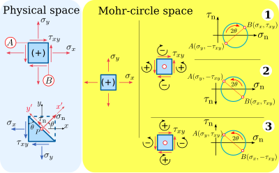
Effigy 5. Engineering science mechanics sign convention for cartoon the Mohr circle. This commodity follows sign-convention # 3, as shown.

In the Mohr-circle-infinite sign convention, normal stresses have the same sign as normal stresses in the physical-infinite sign convention: positive normal stresses act outward to the plane of action, and negative normal stresses act inward to the plane of action.

Shear stresses, however, take a different convention in the Mohr-circle space compared to the convention in the physical infinite. In the Mohr-circle-space sign convention, positive shear stresses rotate the material element in the counterclockwise direction, and negative shear stresses rotate the material in the clockwise direction. This mode, the shear stress component ${\displaystyle \tau _{xy}}$ is positive in the Mohr-circle space, and the shear stress component ${\displaystyle \tau _{yx}}$ is negative in the Mohr-circumvolve space.

Two options exist for drawing the Mohr-circle space, which produce a mathematically right Mohr circle:

1. Positive shear stresses are plotted upwardly (Figure 5, sign convention #1)
2. Positive shear stresses are plotted downward, i.e., the ${\displaystyle \tau _{\mathrm {n} }}$ -axis is inverted (Figure five, sign convention #2).

Plotting positive shear stresses upwardly makes the bending ${\displaystyle ii\theta }$ on the Mohr circle have a positive rotation clockwise, which is opposite to the concrete space convention. That is why some authors^[iii] prefer plotting positive shear stresses downward, which makes the bending ${\displaystyle 2\theta }$ on the Mohr circle have a positive rotation counterclockwise, similar to the physical space convention for shear stresses.

To overcome the "issue" of having the shear stress centrality downward in the Mohr-circle space, there is an alternative sign convention where positive shear stresses are assumed to rotate the material element in the clockwise direction and negative shear stresses are assumed to rotate the cloth element in the counterclockwise management (Figure v, choice 3). This way, positive shear stresses are plotted upward in the Mohr-circle space and the angle ${\displaystyle ii\theta }$ has a positive rotation counterclockwise in the Mohr-circle space. This alternative sign convention produces a circumvolve that is identical to the sign convention #2 in Figure 5 considering a positive shear stress ${\displaystyle \tau _{\mathrm {n} }}$ is besides a counterclockwise shear stress, and both are plotted downwardly. Likewise, a negative shear stress ${\displaystyle \tau _{\mathrm {n} }}$ is a clockwise shear stress, and both are plotted up.

This article follows the technology mechanics sign convention for the physical space and the culling sign convention for the Mohr-circle space (sign convention #3 in Figure five)

Drawing Mohr'due south circumvolve [edit]

Assuming we know the stress components ${\displaystyle \sigma _{x}}$ , ${\displaystyle \sigma _{y}}$ , and ${\displaystyle \tau _{xy}}$ at a point ${\displaystyle P}$ in the object under study, every bit shown in Figure iv, the post-obit are the steps to construct the Mohr circumvolve for the land of stresses at ${\displaystyle P}$ :

1. Draw the Cartesian coordinate system ${\displaystyle (\sigma _{\mathrm {due north} },\tau _{\mathrm {north} })}$ with a horizontal ${\displaystyle \sigma _{\mathrm {due north} }}$ -axis and a vertical ${\displaystyle \tau _{\mathrm {n} }}$ -axis.
2. Plot two points ${\displaystyle A(\sigma _{y},\tau _{xy})}$ and ${\displaystyle B(\sigma _{ten},-\tau _{xy})}$ in the ${\displaystyle (\sigma _{\mathrm {n} },\tau _{\mathrm {n} })}$ space corresponding to the known stress components on both perpendicular planes ${\displaystyle A}$ and ${\displaystyle B}$ , respectively (Figure 4 and half-dozen), following the called sign convention.
3. Describe the diameter of the circumvolve past joining points ${\displaystyle A}$ and ${\displaystyle B}$ with a straight line ${\displaystyle {\overline {AB}}}$ .
4. Draw the Mohr Circle. The centre ${\displaystyle O}$ of the circle is the midpoint of the diameter line ${\displaystyle {\overline {AB}}}$ , which corresponds to the intersection of this line with the ${\displaystyle \sigma _{\mathrm {northward} }}$ centrality.

Finding principal normal stresses [edit]

Stress components on a 2nd rotating element. Instance of how stress components vary on the faces (edges) of a rectangular element as the angle of its orientation is varied. Principal stresses occur when the shear stresses simultaneously disappear from all faces. The orientation at which this occurs gives the principal directions. In this example, when the rectangle is horizontal, the stresses are given past ${\displaystyle \left[{\begin{matrix}\sigma _{xx}&\tau _{xy}\\\tau _{yx}&\sigma _{yy}\end{matrix}}\correct]=\left[{\brainstorm{matrix}-10&10\\10&15\cease{matrix}}\right].}$ The corresponding Mohr's circle representation is shown at the lesser.

The magnitude of the principal stresses are the abscissas of the points ${\displaystyle C}$ and ${\displaystyle E}$ (Figure 6) where the circle intersects the ${\displaystyle \sigma _{\mathrm {n} }}$ -axis. The magnitude of the major principal stress ${\displaystyle \sigma _{1}}$ is always the greatest absolute value of the abscissa of any of these two points. Too, the magnitude of the minor master stress ${\displaystyle \sigma _{2}}$ is always the lowest absolute value of the abscissa of these two points. As expected, the ordinates of these 2 points are zero, corresponding to the magnitude of the shear stress components on the principal planes. Alternatively, the values of the principal stresses tin can be found by

${\displaystyle \sigma _{ane}=\sigma _{\max }=\sigma _{\text{avg}}+R}$

${\displaystyle \sigma _{ii}=\sigma _{\min }=\sigma _{\text{avg}}-R}$

where the magnitude of the average normal stress ${\displaystyle \sigma _{\text{avg}}}$ is the abscissa of the centre ${\displaystyle O}$ , given by

${\displaystyle \sigma _{\text{avg}}={\tfrac {1}{2}}(\sigma _{x}+\sigma _{y})}$

and the length of the radius ${\displaystyle R}$ of the circle (based on the equation of a circle passing through ii points), is given by

${\displaystyle R={\sqrt {\left[{\tfrac {i}{ii}}(\sigma _{10}-\sigma _{y})\right]^{two}+\tau _{xy}^{2}}}}$

Finding maximum and minimum shear stresses [edit]

The maximum and minimum shear stresses represent to the ordinates of the highest and everyman points on the circle, respectively. These points are located at the intersection of the circle with the vertical line passing through the center of the circle, ${\displaystyle O}$ . Thus, the magnitude of the maximum and minimum shear stresses are equal to the value of the circle'south radius ${\displaystyle R}$

${\displaystyle \tau _{\max ,\min }=\pm R}$

Finding stress components on an arbitrary aeroplane [edit]

As mentioned before, later the two-dimensional stress analysis has been performed we know the stress components ${\displaystyle \sigma _{x}}$ , ${\displaystyle \sigma _{y}}$ , and ${\displaystyle \tau _{xy}}$ at a textile bespeak ${\displaystyle P}$ . These stress components act in two perpendicular planes ${\displaystyle A}$ and ${\displaystyle B}$ passing through ${\displaystyle P}$ as shown in Figure 5 and half-dozen. The Mohr circle is used to observe the stress components ${\displaystyle \sigma _{\mathrm {northward} }}$ and ${\displaystyle \tau _{\mathrm {n} }}$ , i.e., coordinates of any point ${\displaystyle D}$ on the circumvolve, acting on any other plane ${\displaystyle D}$ passing through ${\displaystyle P}$ making an angle ${\displaystyle \theta }$ with the plane ${\displaystyle B}$ . For this, two approaches can be used: the double angle, and the Pole or origin of planes.

Double angle [edit]

As shown in Effigy six, to determine the stress components ${\displaystyle (\sigma _{\mathrm {northward} },\tau _{\mathrm {due north} })}$ interim on a plane ${\displaystyle D}$ at an bending ${\displaystyle \theta }$ counterclockwise to the plane ${\displaystyle B}$ on which ${\displaystyle \sigma _{x}}$ acts, we travel an angle ${\displaystyle 2\theta }$ in the aforementioned counterclockwise direction around the circumvolve from the known stress bespeak ${\displaystyle B(\sigma _{x},-\tau _{xy})}$ to point ${\displaystyle D(\sigma _{\mathrm {n} },\tau _{\mathrm {n} })}$ , i.e., an angle ${\displaystyle ii\theta }$ between lines ${\displaystyle {\overline {OB}}}$ and ${\displaystyle {\overline {OD}}}$ in the Mohr circle.

The double angle approach relies on the fact that the angle ${\displaystyle \theta }$ between the normal vectors to any two physical planes passing through ${\displaystyle P}$ (Figure four) is one-half the bending betwixt two lines joining their corresponding stress points ${\displaystyle (\sigma _{\mathrm {due north} },\tau _{\mathrm {n} })}$ on the Mohr circle and the centre of the circle.

This double angle relation comes from the fact that the parametric equations for the Mohr circle are a function of ${\displaystyle 2\theta }$ . It tin also be seen that the planes ${\displaystyle A}$ and ${\displaystyle B}$ in the cloth element effectually ${\displaystyle P}$ of Figure 5 are separated by an bending ${\displaystyle \theta =90^{\circ }}$ , which in the Mohr circle is represented by a ${\displaystyle 180^{\circ }}$ angle (double the bending).

Pole or origin of planes [edit]

Effigy vii. Mohr's circle for airplane stress and airplane strain atmospheric condition (Pole arroyo). Any straight line drawn from the pole volition intersect the Mohr circle at a point that represents the state of stress on a plane inclined at the aforementioned orientation (parallel) in space equally that line.

The second approach involves the determination of a point on the Mohr circle called the pole or the origin of planes. Any straight line fatigued from the pole will intersect the Mohr circle at a betoken that represents the state of stress on a plane inclined at the same orientation (parallel) in space as that line. Therefore, knowing the stress components ${\displaystyle \sigma }$ and ${\displaystyle \tau }$ on any particular plane, i can draw a line parallel to that airplane through the detail coordinates ${\displaystyle \sigma _{\mathrm {n} }}$ and ${\displaystyle \tau _{\mathrm {n} }}$ on the Mohr circle and find the pole as the intersection of such line with the Mohr circumvolve. As an instance, let's assume we have a state of stress with stress components ${\displaystyle \sigma _{10},\!}$ , ${\displaystyle \sigma _{y},\!}$ , and ${\displaystyle \tau _{xy},\!}$ , as shown on Figure 7. First, nosotros can draw a line from point ${\displaystyle B}$ parallel to the airplane of action of ${\displaystyle \sigma _{10}}$ , or, if we choose otherwise, a line from signal ${\displaystyle A}$ parallel to the plane of activity of ${\displaystyle \sigma _{y}}$ . The intersection of any of these ii lines with the Mohr circle is the pole. Once the pole has been determined, to notice the country of stress on a plane making an bending ${\displaystyle \theta }$ with the vertical, or in other words a plane having its normal vector forming an bending ${\displaystyle \theta }$ with the horizontal plane, then we can depict a line from the pole parallel to that plane (See Figure 7). The normal and shear stresses on that plane are then the coordinates of the point of intersection between the line and the Mohr circumvolve.

Finding the orientation of the main planes [edit]

The orientation of the planes where the maximum and minimum principal stresses act, besides known as principal planes, can exist determined by measuring in the Mohr circumvolve the angles ∠BOC and ∠BOE, respectively, and taking half of each of those angles. Thus, the angle ∠BOC between ${\displaystyle {\overline {OB}}}$ and ${\displaystyle {\overline {OC}}}$ is double the bending ${\displaystyle \theta _{p}}$ which the major principal plane makes with airplane ${\displaystyle B}$ .

Angles ${\displaystyle \theta _{p1}}$ and ${\displaystyle \theta _{p2}}$ tin can also be plant from the post-obit equation

${\displaystyle \tan 2\theta _{\mathrm {p} }={\frac {2\tau _{xy}}{\sigma _{y}-\sigma _{x}}}}$

This equation defines two values for ${\displaystyle \theta _{\mathrm {p} }}$ which are ${\displaystyle xc^{\circ }}$ apart (Figure). This equation tin be derived directly from the geometry of the circumvolve, or by making the parametric equation of the circle for ${\displaystyle \tau _{\mathrm {n} }}$ equal to cipher (the shear stress in the principal planes is always zero).

Example [edit]

Assume a textile element nether a land of stress as shown in Figure 8 and Effigy 9, with the plane of one of its sides oriented x° with respect to the horizontal plane. Using the Mohr circle, find:

• The orientation of their planes of activity.
• The maximum shear stresses and orientation of their planes of activity.
• The stress components on a horizontal aeroplane.

Check the answers using the stress transformation formulas or the stress transformation law.

Solution: Post-obit the engineering mechanics sign convention for the concrete space (Figure 5), the stress components for the material element in this instance are:

${\displaystyle \sigma _{x'}=-10{\textrm {MPa}}}$

${\displaystyle \sigma _{y'}=50{\textrm {MPa}}}$

${\displaystyle \tau _{x'y'}=xl{\textrm {MPa}}}$ .

Following the steps for drawing the Mohr circumvolve for this particular state of stress, we start draw a Cartesian coordinate organisation ${\displaystyle (\sigma _{\mathrm {n} },\tau _{\mathrm {due north} })}$ with the ${\displaystyle \tau _{\mathrm {n} }}$ -axis upwardly.

Nosotros then plot two points A(50,twoscore) and B(-10,-40), representing the state of stress at aeroplane A and B as evidence in both Effigy eight and Figure nine. These points follow the engineering science mechanics sign convention for the Mohr-circumvolve infinite (Effigy 5), which assumes positive normals stresses outward from the material chemical element, and positive shear stresses on each aeroplane rotating the textile element clockwise. This way, the shear stress acting on aeroplane B is negative and the shear stress interim on plane A is positive. The diameter of the circle is the line joining indicate A and B. The eye of the circle is the intersection of this line with the ${\displaystyle \sigma _{\mathrm {n} }}$ -axis. Knowing both the location of the centre and length of the diameter, we are able to plot the Mohr circumvolve for this particular state of stress.

The abscissas of both points E and C (Figure 8 and Figure ix) intersecting the ${\displaystyle \sigma _{\mathrm {n} }}$ -axis are the magnitudes of the minimum and maximum normal stresses, respectively; the ordinates of both points E and C are the magnitudes of the shear stresses interim on both the modest and major principal planes, respectively, which is zero for master planes.

Fifty-fifty though the idea for using the Mohr circle is to graphically discover different stress components by really measuring the coordinates for different points on the circle, information technology is more convenient to confirm the results analytically. Thus, the radius and the abscissa of the centre of the circle are

${\displaystyle {\brainstorm{aligned}R&={\sqrt {\left[{\tfrac {i}{2}}(\sigma _{x}-\sigma _{y})\right]^{2}+\tau _{xy}^{2}}}\\&={\sqrt {\left[{\tfrac {1}{2}}(-10-fifty)\right]^{2}+40^{ii}}}\\&=50{\textrm {MPa}}\\\end{aligned}}}$

${\displaystyle {\begin{aligned}\sigma _{\mathrm {avg} }&={\tfrac {1}{ii}}(\sigma _{x}+\sigma _{y})\\&={\tfrac {ane}{ii}}(-10+50)\\&=20{\textrm {MPa}}\\\end{aligned}}}$

and the principal stresses are

${\displaystyle {\begin{aligned}\sigma _{1}&=\sigma _{\mathrm {avg} }+R\\&=seventy{\textrm {MPa}}\\\end{aligned}}}$

${\displaystyle {\begin{aligned}\sigma _{2}&=\sigma _{\mathrm {avg} }-R\\&=-30{\textrm {MPa}}\\\end{aligned}}}$

The coordinates for both points H and M (Figure eight and Effigy 9) are the magnitudes of the minimum and maximum shear stresses, respectively; the abscissas for both points H and G are the magnitudes for the normal stresses acting on the aforementioned planes where the minimum and maximum shear stresses act, respectively. The magnitudes of the minimum and maximum shear stresses can exist institute analytically by

${\displaystyle \tau _{\max ,\min }=\pm R=\pm 50{\textrm {MPa}}}$

and the normal stresses acting on the aforementioned planes where the minimum and maximum shear stresses deed are equal to ${\displaystyle \sigma _{\mathrm {avg} }}$

We tin can cull to either use the double angle approach (Figure viii) or the Pole approach (Figure ix) to notice the orientation of the principal normal stresses and primary shear stresses.

Using the double bending approach nosotros measure the angles ∠BOC and ∠BOE in the Mohr Circle (Figure viii) to notice double the angle the major principal stress and the modest principal stress make with plane B in the physical space. To obtain a more authentic value for these angles, instead of manually measuring the angles, we tin employ the analytical expression

${\displaystyle {\begin{aligned}ii\theta _{\mathrm {p} }=\arctan {\frac {2\tau _{xy}}{\sigma _{ten}-\sigma _{y}}}=\arctan {\frac {2*40}{(-10-50)}}=-\arctan {\frac {four}{iii}}\stop{aligned}}}$

1 solution is: ${\displaystyle ii\theta _{p}=-53.13^{\circ }}$ . From inspection of Effigy 8, this value corresponds to the angle ∠BOE. Thus, the minor principal angle is

${\displaystyle \theta _{p2}=-26.565^{\circ }}$

Then, the major master angle is

${\displaystyle {\brainstorm{aligned}ii\theta _{p1}&=180-53.xiii^{\circ }=126.87^{\circ }\\\theta _{p1}&=63.435^{\circ }\\\terminate{aligned}}}$

Remember that in this particular example ${\displaystyle \theta _{p1}}$ and ${\displaystyle \theta _{p2}}$ are angles with respect to the plane of activeness of ${\displaystyle \sigma _{10'}}$ (oriented in the ${\displaystyle x'}$ -axis)and non angles with respect to the plane of action of ${\displaystyle \sigma _{x}}$ (oriented in the ${\displaystyle x}$ -axis).

Using the Pole approach, we first localize the Pole or origin of planes. For this, we draw through signal A on the Mohr circle a line inclined ten° with the horizontal, or, in other words, a line parallel to plane A where ${\displaystyle \sigma _{y'}}$ acts. The Pole is where this line intersects the Mohr circle (Figure 9). To confirm the location of the Pole, we could draw a line through point B on the Mohr circle parallel to the aeroplane B where ${\displaystyle \sigma _{10'}}$ acts. This line would also intersect the Mohr circle at the Pole (Figure 9).

From the Pole, we depict lines to different points on the Mohr circle. The coordinates of the points where these lines intersect the Mohr circle indicate the stress components acting on a plane in the physical space having the same inclination as the line. For example, the line from the Pole to indicate C in the circle has the same inclination as the plane in the concrete space where ${\displaystyle \sigma _{ane}}$ acts. This plane makes an angle of 63.435° with plane B, both in the Mohr-circle space and in the physical infinite. In the same fashion, lines are traced from the Pole to points E, D, F, G and H to find the stress components on planes with the same orientation.

Mohr's circumvolve for a full general three-dimensional country of stresses [edit]

Effigy 10. Mohr's circle for a three-dimensional state of stress

To construct the Mohr circle for a general three-dimensional case of stresses at a point, the values of the primary stresses ${\displaystyle \left(\sigma _{1},\sigma _{2},\sigma _{3}\right)}$ and their principal directions ${\displaystyle \left(n_{one},n_{2},n_{3}\right)}$ must be first evaluated.

Considering the primary axes as the coordinate system, instead of the general ${\displaystyle x_{ane}}$ , ${\displaystyle x_{ii}}$ , ${\displaystyle x_{iii}}$ coordinate system, and assuming that ${\displaystyle \sigma _{ane}>\sigma _{2}>\sigma _{3}}$ , and so the normal and shear components of the stress vector ${\displaystyle \mathbf {T} ^{(\mathbf {n} )}}$ , for a given plane with unit vector ${\displaystyle \mathbf {due north} }$ , satisfy the following equations

${\displaystyle {\brainstorm{aligned}\left(T^{(n)}\right)^{2}&=\sigma _{ij}\sigma _{ik}n_{j}n_{k}\\\sigma _{\mathrm {n} }^{2}+\tau _{\mathrm {due north} }^{two}&=\sigma _{1}^{2}n_{1}^{2}+\sigma _{2}^{ii}n_{2}^{2}+\sigma _{three}^{ii}n_{iii}^{2}\end{aligned}}}$

${\displaystyle \sigma _{\mathrm {northward} }=\sigma _{1}n_{one}^{2}+\sigma _{2}n_{ii}^{2}+\sigma _{three}n_{3}^{2}.}$

Knowing that ${\displaystyle n_{i}n_{i}=n_{1}^{2}+n_{2}^{2}+n_{three}^{2}=1}$ , we can solve for ${\displaystyle n_{1}^{2}}$ , ${\displaystyle n_{2}^{2}}$ , ${\displaystyle n_{three}^{two}}$ , using the Gauss elimination method which yields

${\displaystyle {\begin{aligned}n_{i}^{two}&={\frac {\tau _{\mathrm {northward} }^{2}+(\sigma _{\mathrm {n} }-\sigma _{2})(\sigma _{\mathrm {n} }-\sigma _{iii})}{(\sigma _{1}-\sigma _{2})(\sigma _{1}-\sigma _{3})}}\geq 0\\n_{2}^{ii}&={\frac {\tau _{\mathrm {n} }^{2}+(\sigma _{\mathrm {n} }-\sigma _{3})(\sigma _{\mathrm {north} }-\sigma _{1})}{(\sigma _{2}-\sigma _{3})(\sigma _{2}-\sigma _{1})}}\geq 0\\n_{3}^{2}&={\frac {\tau _{\mathrm {n} }^{2}+(\sigma _{\mathrm {n} }-\sigma _{1})(\sigma _{\mathrm {north} }-\sigma _{ii})}{(\sigma _{3}-\sigma _{1})(\sigma _{3}-\sigma _{2})}}\geq 0.\finish{aligned}}}$

Since ${\displaystyle \sigma _{1}>\sigma _{2}>\sigma _{3}}$ , and ${\displaystyle (n_{i})^{2}}$ is not-negative, the numerators from these equations satisfy

${\displaystyle \tau _{\mathrm {n} }^{2}+(\sigma _{\mathrm {n} }-\sigma _{ii})(\sigma _{\mathrm {due north} }-\sigma _{3})\geq 0}$ every bit the denominator ${\displaystyle \sigma _{one}-\sigma _{2}>0}$ and ${\displaystyle \sigma _{1}-\sigma _{3}>0}$

${\displaystyle \tau _{\mathrm {north} }^{2}+(\sigma _{\mathrm {n} }-\sigma _{3})(\sigma _{\mathrm {n} }-\sigma _{1})\leq 0}$ every bit the denominator ${\displaystyle \sigma _{2}-\sigma _{three}>0}$ and ${\displaystyle \sigma _{2}-\sigma _{1}<0}$

${\displaystyle \tau _{\mathrm {n} }^{two}+(\sigma _{\mathrm {due north} }-\sigma _{1})(\sigma _{\mathrm {n} }-\sigma _{2})\geq 0}$ as the denominator ${\displaystyle \sigma _{3}-\sigma _{1}<0}$ and ${\displaystyle \sigma _{3}-\sigma _{2}<0.}$

These expressions can exist rewritten as

${\displaystyle {\begin{aligned}\tau _{\mathrm {n} }^{2}+\left[\sigma _{\mathrm {n} }-{\tfrac {1}{2}}(\sigma _{ii}+\sigma _{3})\right]^{2}\geq \left({\tfrac {i}{2}}(\sigma _{2}-\sigma _{3})\right)^{2}\\\tau _{\mathrm {due north} }^{2}+\left[\sigma _{\mathrm {north} }-{\tfrac {1}{2}}(\sigma _{1}+\sigma _{iii})\right]^{2}\leq \left({\tfrac {1}{2}}(\sigma _{1}-\sigma _{three})\correct)^{2}\\\tau _{\mathrm {n} }^{2}+\left[\sigma _{\mathrm {n} }-{\tfrac {1}{2}}(\sigma _{one}+\sigma _{2})\right]^{ii}\geq \left({\tfrac {one}{2}}(\sigma _{1}-\sigma _{2})\right)^{2}\\\end{aligned}}}$

which are the equations of the three Mohr's circles for stress ${\displaystyle C_{one}}$ , ${\displaystyle C_{2}}$ , and ${\displaystyle C_{3}}$ , with radii ${\displaystyle R_{one}={\tfrac {i}{2}}(\sigma _{ii}-\sigma _{three})}$ , ${\displaystyle R_{2}={\tfrac {1}{2}}(\sigma _{i}-\sigma _{iii})}$ , and ${\displaystyle R_{3}={\tfrac {1}{2}}(\sigma _{1}-\sigma _{2})}$ , and their centres with coordinates ${\displaystyle \left[{\tfrac {1}{2}}(\sigma _{2}+\sigma _{3}),0\right]}$ , ${\displaystyle \left[{\tfrac {ane}{2}}(\sigma _{1}+\sigma _{3}),0\right]}$ , ${\displaystyle \left[{\tfrac {1}{ii}}(\sigma _{ane}+\sigma _{ii}),0\right]}$ , respectively.

These equations for the Mohr circles testify that all admissible stress points ${\displaystyle (\sigma _{\mathrm {north} },\tau _{\mathrm {northward} })}$ lie on these circles or within the shaded area enclosed by them (see Figure x). Stress points ${\displaystyle (\sigma _{\mathrm {n} },\tau _{\mathrm {north} })}$ satisfying the equation for circle ${\displaystyle C_{1}}$ lie on, or outside circle ${\displaystyle C_{ane}}$ . Stress points ${\displaystyle (\sigma _{\mathrm {due north} },\tau _{\mathrm {n} })}$ satisfying the equation for circumvolve ${\displaystyle C_{2}}$ prevarication on, or inside circle ${\displaystyle C_{ii}}$ . And finally, stress points ${\displaystyle (\sigma _{\mathrm {n} },\tau _{\mathrm {n} })}$ satisfying the equation for circle ${\displaystyle C_{iii}}$ prevarication on, or outside circumvolve ${\displaystyle C_{three}}$ .

See likewise [edit]

• Critical plane analysis

References [edit]

1. ^ "Chief stress and principal plane". www.engineeringapps.net . Retrieved 2019-12-25 .
2. ^ Parry, Richard Hawley Gray (2004). Mohr circles, stress paths and geotechnics (2 ed.). Taylor & Francis. pp. i–30. ISBN0-415-27297-1.
3. ^ Gere, James M. (2013). Mechanics of Materials. Goodno, Barry J. (eighth ed.). Stamford, CT: Cengage Learning. ISBN9781111577735.

Bibliography [edit]

• Beer, Ferdinand Pierre; Elwood Russell Johnston; John T. DeWolf (1992). Mechanics of Materials . McGraw-Colina Professional. ISBN0-07-112939-1.
• Brady, B.H.G.; East.T. Brown (1993). Stone Mechanics For Hole-and-corner Mining (Third ed.). Kluwer Academic Publisher. pp. 17–29. ISBN0-412-47550-2.
• Davis, R. O.; Selvadurai. A. P. Southward. (1996). Elasticity and geomechanics. Cambridge University Press. pp. 16–26. ISBN0-521-49827-9.
• Holtz, Robert D.; Kovacs, William D. (1981). An introduction to geotechnical engineering. Prentice-Hall civil applied science and technology mechanics serial. Prentice-Hall. ISBN0-13-484394-0.
• Jaeger, John Conrad; Melt, N.Thou.W.; Zimmerman, R.W. (2007). Fundamentals of stone mechanics (Fourth ed.). Wiley-Blackwell. pp. 9–41. ISBN978-0-632-05759-7.
• Jumikis, Alfreds R. (1969). Theoretical soil mechanics: with practical applications to soil mechanics and foundation engineering. Van Nostrand Reinhold Co. ISBN0-442-04199-3.
• Parry, Richard Hawley Greyness (2004). Mohr circles, stress paths and geotechnics (2 ed.). Taylor & Francis. pp. 1–30. ISBN0-415-27297-1.
• Timoshenko, Stephen P.; James Norman Goodier (1970). Theory of Elasticity (3rd ed.). McGraw-Loma International Editions. ISBN0-07-085805-5.
• Timoshenko, Stephen P. (1983). History of strength of materials: with a brief account of the history of theory of elasticity and theory of structures. Dover Books on Physics. Dover Publications. ISBN0-486-61187-six.

External links [edit]

• Mohr's Circumvolve and more circles past Rebecca Brannon
• DoITPoMS Education and Learning Package- "Stress Analysis and Mohr's Circle"

Source: https://en.wikipedia.org/wiki/Mohr%27s_circle

Posted by: ruizwarsted.blogspot.com

Share this post